Recently, RNA-velocity estimation has becomes increasingly popular tool in single-cell RNA seq analysis. In this post, we will discuss an additional advantage brought by the Unspliced-Spliced-Ambiguous (USA) mode introduced in alevin-fry 0.3.0 and later. That is, the solution presented in that approach for controlling the spurious mapping to spliced transcripts of sequenced fragments arising from introns (in the absence of full decoy) basically gives us the preprocessing results we need to perform an RNA-velocity analysis “for free”. Here we provide an end-to-end tutorial describing how to perform an RNA-velocity analysis for a 10x Chromium dataset. In this tutorial, we will show the whole analysis pipeline, starting from the raw FASTQ files to the gorgeous velocity plots (generated by scVelo) that you may like to include in your next analysis or paper.

Preliminaries and overview of the pipeline

For this pipeline, you will need salmon (>= v1.5.0), and alevin-fry (>= v0.3.0). As always, it’s best to use as recent versions of these tools as possible. To prepare the reference spliced+intron (splici) transcriptome, you will need a recent version of R and the packages roe. Alternatively, if you are a Python lover, you can use pyroe to prepare the splici reference. Having bedtools installed will make pyroe run faster. gffread CLI is needed for converting genes’ Entrez ID to the official gene name. To infer the RNA-velocity, you will need scVelo python package and its dependencies installed.

If you use conda or anaconda, you can configure the environment by running the follow command in your terminal:

conda install -c Bioconda salmon alevin-fry pyroe scVelo gffread bedtools

Downloading Dataset

In this tutorial, we will use a mouse pancreas experiment data introduced by Bastidas-Ponce et al. 2019, GEO accession GSE132188, as a real world example. A subset of this dataset is included in the scVelo python package as a built-in example dataset (below we will call it the scVelo dataset). Here we will start with the raw FASTQ file downloaded from GEO, and walk through the RNA-velocity analysis pipeline until the generation of the velocity graph using scVelo.

To download the dataset from GEO, make sure that there is at least 30GB free space in your disk, and open your terminal to run:

$ mkdir af_tutorial_velocity
$ cd af_tutorial_velocity
$ mkdir data
$ cd data
$ wget ftp://ftp.sra.ebi.ac.uk/vol1/fastq/SRR920/004/SRR9201794/SRR9201794_1.fastq.gz
$ wget ftp://ftp.sra.ebi.ac.uk/vol1/fastq/SRR920/004/SRR9201794/SRR9201794_2.fastq.gz

Preparing the splici reference

Following our USA mode tutorial, we build the splici reference over the mouse transcriptome.

Obtaining the reference sequeneces and GTF

First we obtain the pre-built reference sequences and GTF from 10X Genomics. You can also choose to build it on your own by following this note.

$ wget http://cf.10xgenomics.com/supp/cell-exp/refdata-cellranger-mm10-2.1.0.tar.gz
$ tar xvf refdata-cellranger-mm10-2.1.0.tar.gz

making the splici refernece

We provide the function make_splici_txome() for making splici reference both in the roe R package and pyroe python package. Here we show the example of making splici reference in both ways.

making the splici reference using roe in R

The roe R package provides useful functions for assisting alevin-fry to process single-cell data. However, if we just want to make a splici reference, usefulaf provides a Rscript for making the splici refernce in command line using roe. This script will install roe for you if it is not installed.

First of all, we should pull the Rscript from usefulaf

$ wget https://raw.githubusercontent.com/COMBINE-lab/usefulaf/main/R/build_splici_ref.R

or you can right click here to save it to your PC directly.

Then, we can execute this Rscript to make the splici reference in terminal.

$ Rscript build_splici_ref.R \
refdata-cellranger-mm10-2.1.0/fasta/genome.fa \
refdata-cellranger-mm10-2.1.0/genes/genes.gtf \
151 mm10_2.1.0_splici_fl146 \
--flank-trim-length 5 --filename-prefix splici

$ ls mm10_2.1.0_splici_fl146

Run Rscript build_splici_ref.R -h for full usage.

Sometimes one of the dependencies will return warnings and errors when running this command, but as long as you see Done. before the Warning messages, the command ran successfully. Or, you can also check whether the following files show up:

$ ls mm10_2.1.0_splici_fl146
splici_fl146.fa  splici_fl146_t2g_3col.tsv

If you would like to make a splici reference interactively in R, first make sure that roe is installed, follow this instruction if haven’t. Then, click to see the R code for making a splici reference interactively in R.

making splici refernce using pyroe

It is even more convinent to make splici reference using pyroe! If you haven’t install pyroe, you can install it via bioconda or pip. Note : to make pyroe work more quickly, it is recommended to have the latest version of bedtools (Aaron R. Quinlan and Ira M. Hall, 2010) installed. You can do this via conda or follow this to install it.

Then, you can call pyroe to make splici in terminal without launching python:

$ pyroe make-splici \
refdata-cellranger-mm10-2.1.0/fasta/genome.fa \
refdata-cellranger-mm10-2.1.0/genes/genes.gtf \
151 mm10_2.1.0_splici_fl146 \
--flank-trim-length 5 --filename-prefix splici

$ ls mm10_2.1.0_splici_fl146

Run pyroe make-splici -h for full usage.

If it runs successfully, you will see the following output of the ls command call:

$ ls mm10_2.1.0_splici_fl146
splici_fl146.fa  splici_fl146_t2g_3col.tsv

make gene ID to gene name mapping file

Finally, before we leave the data folder, let’s get the Entrez gene ID to gene name mapping. If you haven’t installed gffread, you can do this via conda or follow this.

$ gffread refdata-cellranger-mm10-2.1.0/genes/genes.gtf -o refdata-cellranger-mm10-2.1.0/genes/genes.gff
$ grep "gene_name" refdata-cellranger-mm10-2.1.0/genes/genes.gff | cut -f9 | cut -d';' -f2,3 | sed 's/=/ /g' | sed 's/;/ /g' | cut -d' ' -f2,4 | sort | uniq > mm10-2.1.0_geneid_to_name.txt

Building the salmon/alevin splici index

Now, we will build the index:

$ cd ..
$ salmon index -t data/mm10-2.1.0_splici_fl146/splici_fl146.fa -i mm10-2.1.0_splici_fl146_idx -p 16

The -p 16 flag tells salmon to use multiple threads (16 here) during indexing. While not all steps of indexing are multi-threaded, many are, and this will speed up index construction substantially.

Mapping the data to obtain a RAD file

Now that we have downloaded the data and indexed the splici reference, we are ready to map our reads. We will be using sketch mode which uses pseudoalignment with structural constraints to generate a RAD file (a chunk-oriented binary (Reduced Alignment Data) file storing the information necessary for subsequent phases of processing). We can do this as follows:

$ salmon alevin -i mm10-2.1.0_splici_fl146_idx -p 16 -l ISR --chromium --sketch \
-1 data/SRR9201794_1.fastq.gz \
-2 data/SRR9201794_2.fastq.gz \
-o pancreas_map

This will produce an output folder called pancreas_map that contains all of the information that we need to process the mapped reads (1).

Processing the mapped reads

Keep following our USA-mode tutorial, we then run alevin-fry to generate permit list, collate corrected cells and do quantification. Notice that when running alevin-fry quant command we use a 3-column tx2gene file, which contains the ID of each reference sequence (Entrez transcript ID in this case), their correspoindg gene ID, and their splicing status (either spliced (S) or unspliced (U))). When detected a 3-column tx2gene file, alevin-fry will automatically enter its USA mode to execute splice-status-aware quantification.

$ alevin-fry generate-permit-list -d fw -k -i pancreas_map -o pancreas_quant
$ alevin-fry collate -t 16 -i pancreas_quant -r pancreas_map
$ alevin-fry quant -t 16 -i pancreas_quant -o pancreas_quant_res --tg-map data/mm10_2.1.0_splici_fl146/splici_fl146_t2g_3col.tsv --resolution cr-like --use-mtx

The output

After ran this command, the resulting quantification information can be found in pbmc_10k_v3_quant_res/ folder. Crucially, this entire directory will be important for the functions we provide below, so please keep its structure intact. Within this directory, there are some metadata files, including one actually named meta_info.json. If you look in this file, you’ll see something like the following:

{
  "alt_resolved_cell_numbers": [],
  "dump_eq": false,
  "num_genes": 86076,
  "num_quantified_cells": 11736,
  "resolution_strategy": "CellRangerLike",
  "usa_mode": true
}

The usa_mode flag says that our data was processed in Unspliced-Spliced-Ambiguous mode. This happened since the transcript-to-gene mapping we provided, t2g_3col.tsv, had 3 columns instead of 2, to allow specifying the splicing state of each transcript.

Within this directory, there is a subdirectory named alevin with 3 files: quants_mat.mtx, quants_mat_cols.txt, and quants_mat_rows.txt which correspond, respectively, to the count matrix, the gene names for each column of this matrix, and the corrected, filtered cell barcodes for each row of this matrix. Importantly, the dimensions of this matrix will be num_cells x 3num_genes — the factor of 3 arises because this quantification mode separately attributes UMIs to _spliced, or unspliced (in this case, intronic) gene sequence, or as ambiguous (not able to be confidently assigned to the spliced or unspliced category). All of these counts are packed into the same output matrix. The first num_genes columns correspond to the spliced counts, the next num_genes columns correspond to the unspliced counts, and the final num_genes columns correspond to the ambiguous counts. Sound compicated? Don’t worry, the loadFry() function in the fishpond R package and

RNA velocity estimation

Subsequent velocity estimation is done using scVelo. We will also show that, when using same set of genes and cells as in the scVelo tutorial, the velocity graph generated from the alevin-fry count matrix (below we call it as the fry dataset) is very similar to the scVelo tutorial output, even though these two datasets are generated by completely different toolchains.

First, we’ll load our favorite Python environment; you can use IPython, or a Jupyter notebook.

processing the count matrix

We load the packages we will use in the following procedure.

import numpy as np
import pandas as pd
import scanpy as sc
import anndata
import scvelo as scv
import matplotlib
import scipy
from pyroe import load_fry
import os

We then process the count matrix generated by alevin-fry:

frydir = "pancreas_quant_res"
e2n_path = "data/mm10-2.1.0_geneid_to_name.txt"
adata = load_fry(frydir, output_format = "velocity")
e2n = dict([ l.rstrip().split() for l in open(e2n_path).readlines()])
adata.var_names = [e2n[e] for e in adata.var_names]

When using the “velocity” output format, we use S+A as the spliced counts, and U as the unsplcied counts. This strategy is widely adopted by other tools and makes the assumption that ambiguous UMIs are most likely to derive from spliced transcripts. In this data, ambiguous counts make up only 4% of the total deduplicated UMIs. We tested many strategies to assign ambiguous count, and we found that as long as the rule of assigning ambiguous count relates to the proportion of S to U, the velocity graph undergoes only small changes.

Run scVelo

With the AnnData object with the spliced and unspliced layers in hand, we can run scVelo to generate the velocity graph. scVelo provides multiple modes when calculating velocity, here we use the dynamical mode as an example.

# make sure gene names are unique
adata.var_names_make_unique()

# get embeddings
sc.tl.pca(adata)
sc.pp.neighbors(adata)
sc.tl.tsne(adata)
sc.tl.umap(adata, n_components = 2)

# housekeeping
matplotlib.use('AGG')
scv.settings.set_figure_params('scvelo')

# get the proportion of spliced and unspliced count
scv.utils.show_proportions(adata)

# filter cells and genes, then normalize expression values
scv.pp.filter_and_normalize(adata, min_shared_counts=20, n_top_genes=2000,enforce=True)

# scVelo pipeline
scv.pp.moments(adata, n_pcs=30, n_neighbors=30)
scv.tl.recover_dynamics(adata, n_jobs = 11)
scv.tl.velocity(adata, mode = 'dynamical')
scv.tl.velocity_graph(adata)
adata.write('pancreas_full_dim_scvelo.h5ad', compression='gzip')
scv.pl.velocity_embedding_stream(adata, basis='X_umap', save="pancreas_full_dim.png")

The velocity graph is under the figure folder of the working directory.

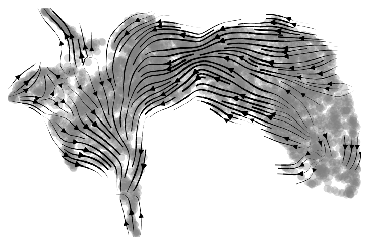Fig 1. Velocity graph of the alevin-fry dataset.

Utilizing the cell type annotation provided by scVelo

The scvelo dataset contains cell type annotation information, which is very nice to show in the velocity graph. However, the scVelo dataset has fewer genes and cells than the fry dataset, probably becauase we used a slightly different version of reference transcriptome. So, we do an intersection of the two dataset to implant the annotation information from the scVelo dataset to our fry dataset.

# create adata
adata = anndata.AnnData(X = spliced, 
                        layers = dict(spliced = spliced, 
                                    unspliced = unspliced))

# assign obs_names(cell IDs) and var_names(gene names)
adata.obs_names = obs_names
adata.var_names = var_names
adata.var_names_make_unique()

example_adata = scv.datasets.pancreas()
subset_adata = adata[example_adata.obs_names, np.intersect1d(example_adata.var_names, adata.var_names)]
example_adata = example_adata[subset_adata.obs_names, subset_adata.var_names]
subset_adata.obs = example_adata.obs
subset_adata.obsm["X_umap"] = example_adata.obsm["X_umap"]

# housekeeping
matplotlib.use('AGG')
scv.settings.set_figure_params('scvelo')

# get the proportion of spliced and unspliced count
scv.utils.show_proportions(subset_adata)

# filter cells and genes, then normalize expression values
scv.pp.filter_and_normalize(subset_adata, min_shared_counts=20, n_top_genes=2000,enforce=True)

# scVelo pipeline
scv.pp.moments(subset_adata, n_pcs=30, n_neighbors=30)
scv.tl.recover_dynamics(subset_adata, n_jobs = 11)
scv.tl.velocity(subset_adata, mode = 'dynamical')
scv.tl.velocity_graph(subset_adata)
subset_adata.write('pancreas_trimmed_scvelo.h5ad', compression='gzip')
scv.pl.velocity_embedding_stream(subset_adata, basis='X_umap', save="pancreas_trimmed.png")

By doing so, the velocity grpah generated is colored by the cell type annotation. As we can see, using the same cells and genes and UMAP embedding, this velocity graph very similar to the one shown in scVelo’s tutorial.

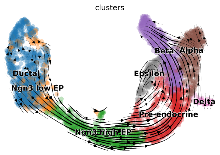Fig 2. Velocity graph of alevin-fry dataset using scVelo provided cell type annotation and UMAP embedding.

Summary

In this tutorial, we’ve demonstrate an end-to-end pipeline using the USA (Unspliced/Spliced/Ambiguous) mode of alevin-fry for performing RNA-velocity analysis. In this mode, alevin-fry genearate three counts for each gene within each cell, which represent the confidently unspliced count, the confidently spliced count and the ambiguous count. The scVelo package desired AnnData object can be easily generated using these three count matrices. We further show that, if we only include the cells and genes that are used in the scVelo dataset, which comes from the same raw data as the fry dataset, the velocity graph generated by the scVelo dataset and the fry dataset are very similar. This shows that alevin-fry’s USA mode — initially designed to avoid the problem of spuriously attributing UMIs arising from unspliced transcripts to (spliced) gene expression — has the ability to accurately infer the spliced and the unspliced counts for the genes in a given scRNA-seq experiment. Hence, processing your data in USA-mode gives the input necessary for subsequent RNA-velocity analysis “for free”!

Notes

• A complete version of the scVelo related code can be found at here.
• This tutorial is primarily the work of Dongze He. We would also like to thank Charlotte Soneson for providing valuable feedback on the proposed pipeline and code.