As the number of different tools available to enable versatile and efficient pre-processing of single-cell and single-nucleus RNA-seq data continues to increase, the trade-offs of different approaches to pre-processing are starting to be explored in more detail. For example, one of the high-level results reported in the recent pre-print for the STARsolo tool is that “Pseudoalignment-to-transcriptome predicts expression for thousands of non-expressed genes”. This is unfortunate to the extent that such methods are the fastest and require the least working memory to preprocess single-cell experiments. While more investigation is certainly warranted into the exact mechanisms that lead to the prediction of expression for these genes, and the extent to which they might affect subsequent analysis, one of the primary mechanisms posited is spurious pseudoalignment of sequenced fragments that truly arise from intronic sequences, rather than from spliced, mature mRNA. Given these observations, the question naturally arises, “Can these spuriously mapped fragments be controlled for without forfeiting all of the resource advantages of pseudoalignment-to-transcriptome?”.

Gladly, the answer to this question appears to be yes. In this tutorial we describe an approach to this problem, using alevin-fry, that largely addresses the issue of spurious expression arising from mapping errors, while maintaining the speed advantages and only somewhat compromising on memory usage (the modified index we use can be built and mapped against using a machine with <16GB of RAM). The core of the strategy described here will to be to construct an index that consists of both spliced mRNA transcripts as well as intronic sequences (with appropriately-sized flanking regions), as is often done when performing RNA-velocity preprocessing with transcriptome-oriented approaches. We will refer to this type of reference below as a splici (for spliced+intron) index.

Preliminaries and overview of the pipeline

For this pipeline, you will need salmon (>= v1.4.0), and alevin-fry (>= v0.3.0). As always, it’s best to use as recent versions of these tools as possible. To prepare the reference spliced+intron (splici) transcriptome, you will need a recent version of R and the packages eisaR, Biostrings and BSgenome.

Preparing the splici reference

In this pipeline, we will be processing the PBMC10k v3 data made available by 10x Genomics. This will require us to build the splici reference over the human transcriptome. To do this, we will largely follow the process outlined in the eisaR vignette.

Obtaining the reference sequeneces and GTF

We will use the latest Human reference (GRCh38) dataset from 10x.

$ wget https://cf.10xgenomics.com/supp/cell-exp/refdata-gex-GRCh38-2020-A.tar.gz
$ tar xzf refdata-gex-GRCh38-2020-A.tar.gz

Now, we’ll move into this directory to prepare the splici reference:

$ cd refdata-gex-GRCh38-2020-A

and we’ll launch into R to do the actual processing

$ R

click to see the R function for making splici transcriptome (provided as a Gist), this function needs to be pasted into R will be used in the following R code:

After pasted the above function into R, please run the following code in R:

suppressPackageStartupMessages({
  library(eisaR)
  library(Biostrings)
  library(BSgenome)
  library(stringr)
  library(GenomicFeatures)
})

gtf_path = file.path( "genes/genes.gtf")
genome_path = file.path( "fasta/genome.fa")
read_length = 91
flank_trim_length = 5
output_dir = paste0("transcriptome_splici_fl", read_length - flank_trim_length)

make_splici_txome(gtf_path=gtf_path, 
                  genome_path=genome_path, 
                  read_length=read_length, 
                  flank_trim_length=flank_trim_length, 
                  output_dir=output_dir)

Building the salmon/alevin splici index

Now, we will make the working directory for our analysis and build the index:

$ cd ..
$ mkdir -p af_tutorial_splici
$ cd af_tutorial_splici
$ salmon index -t ../refdata-gex-GRCh38-2020-A/transcriptome_splici_fl86/transcriptome_splici_fl86.fa -i grch38_splici_idx -p 16

The -p 16 flag tells salmon to use multiple threads during indexing. While not all steps of indexing are multi-threaded, many are, and this will speed up index construction substantially.

Obtaining the read data

Now we will download the sequencing data. This is the same data used in this alevin-fry tutorial, but we will repeat here the steps of how to obtain this data.

This is a tagged-end single-cell dataset that makes use of version 3 of the 10x chromium chemistry. First download the raw FASTQ files (that you can obtain here).

$ wget https://cg.10xgenomics.com/samples/cell-exp/3.0.0/pbmc_10k_v3/pbmc_10k_v3_fastqs.tar

$ tar xf pbmc_10k_v3_fastqs.tar

now you should be able to list the files as such, and see the following:

$ ls pbmc_10k_v3_fastqs/
10xv3_whitelist.txt
pbmc_10k_v3_S1_L001_R1_001.fastq.gz
pbmc_10k_v3_S1_L002_I1_001.fastq.gz
pbmc_10k_v3_S1_L002_R2_001.fastq.gz
pbmc_10k_v3_S1_L001_I1_001.fastq.gz
pbmc_10k_v3_S1_L001_R2_001.fastq.gz
pbmc_10k_v3_S1_L002_R1_001.fastq.gz

Mapping the data to obtain a RAD file

Now that we have downloaded the data and indexed the reference, we are ready to map our reads. We will be using sketch mode which uses pseudoalignment with structural constraints to generate a RAD file (a chunk-oriented binary (Reduced Alignment Data) file storing the information necessary for subsequent phases of processing). We can do this as follows:

$ salmon alevin -i grch38_splici_idx -p 16 -l IU --chromiumV3 --sketch \
-1 pbmc_10k_v3_fastqs/pbmc_10k_v3_S1_L001_R1_001.fastq.gz \
pbmc_10k_v3_fastqs/pbmc_10k_v3_S1_L002_R1_001.fastq.gz \
-2 pbmc_10k_v3_fastqs/pbmc_10k_v3_S1_L001_R2_001.fastq.gz \
pbmc_10k_v3_fastqs/pbmc_10k_v3_S1_L002_R2_001.fastq.gz \
-o pbmc_10k_v3_map \
--tgMap t2g.tsv

This will produce an output folder called pbmc_10k_v3_map that contains all of the information that we need to process the mapped reads ⁽¹⁾.

Processing the mapped reads

Generating a permit list of filtered cells

The next step in the pipeline is to generate a “permit list” of barcodes that are believed to belong to real (high-quality) cells. Many of the barcodes that appear in the mapping file will contain only a handful of reads, and therefore are very unlikely to correspond to droplets containing a cell. Given that alevin-fry works by converting the raw mapping file into a mapping file where read mappings are collated by corrected barcode and chunked within the file on a per-cell basis, providing a filtered permit list is an important step in the subsequent processing of the data.

The alevin-fry tool provides a number of different ways to generate a permit list (here we will use the knee method). One can also force it to extract a given number (k) of cells (it will sort and take the k most frequent barcodes), give an expected number of cells (where it will estimate the number of barcodes to include using the same algorithm as STARsolo), provide it with an explicit list of filtered cell barcodes (using the -b option), or as of alevin-fry v0.2.0, perform unfiltered quantification the full list of potentially valid barcodes (like the 10xv3_whitelist.txt in our pbmc_10k_v3_fastqs directory) using the -u option ⁽²⁾. Performing unfiltered quantification will attempt to quantify every barcode that is present in the data, even if they are unlikely to correspond to a live captured cell. Thus, if using such an approach, it is important to filter the resulting quantification matrix downstream before subsequent analysis using a method like Empty Drops if you are analyzing your data with R, or scanpy’s filter_cells (if you are analyzing your data with python).

Rather than repeat redundant descriptions from other tutorials, we will instead briefly summarize the steps below until the analysis differs.

First, we generate the permit list using the knee method, and filtering the mappings to retain those that match the underlying reference in the forward (-d fw) orientation:

$ alevin-fry generate-permit-list -d fw -k -i pbmc_10k_v3_map -o pbmc_10k_v3_quant

Collating the file

Next, we will collate the input RAD file. One potentially useful feature introduced in alevin-fry 0.3.0 is the ability to optionally compress the output (collated RAD file). If you wish to do this, you can provide the flag --compress to the command below; none of the subsequent steps will change.

$ alevin-fry collate -t 16 -i pbmc_10k_v3_quant -r pbmc_10k_v3_map

Quantifying UMIs per-gene and per-cell

The last pre-processing step we will complete with alevin-fry is to generate a cell-by-gene count matrix from the collated mapping file. Just as with the initial mapping and permit-listing, there are a number of different options one can choose for the algorithm used to resolve UMIs. However, here, since we are using the Unspliced-Spliced-Ambiguous (USA) mode to separately keep track of the types of transcripts from which UMIs are sampled, we will have to use the cr-like resolution method. Currently, this is the only method supported when performing USA quantification, though other resolution strategies will be implemented for this mode in the future.

$ alevin-fry quant -t 16 -i pbmc_10k_v3_quant -o pbmc_10k_v3_quant_res --tg-map ../refdata-gex-GRCh38-2020-A/transcriptome_splici_fl86/transcriptome_splici_fl86_t2g_3col.tsv --resolution cr-like --use-mtx

The output

After running this command, the resulting quantification information can be found in pbmc_10k_v3_quant_res/. Crucially, this entire directory will be important for the functions we provide below, so please keep its structure intact. Within this directory, there are some metadata files, including one actually named meta_info.json. If you look in this file, you’ll see something like the following:

{
  "alt_resolved_cell_numbers": [],
  "dump_eq": false,
  "num_genes": 109803,
  "num_quantified_cells": 11256,
  "resolution_strategy": "CellRangerLike",
  "usa_mode": true
}

The usa_mode flag says that our data was processed in unspliced-spliced-ambiguous mode. This happened since the transcript-to-gene mapping we provided had 3 columns instead of 2, to allow specifying the splicing state of each transcript.

Within this directory, there is a subdirectory named alevin with 3 files: quants_mat.mtx, quants_mat_cols.txt, and quants_mat_rows.txt which correspond, respectively, to the count matrix, the gene names for each column of this matrix, and the corrected, filtered cell barcodes for each row of this matrix. Importantly, the dimensions of this matrix will be num_cells x 3num_genes — the factor of 3 arises because this quantification mode separately attributes UMIs to *spliced, or unspliced (in this case, intronic) gene sequence, or as ambiguous (not able to be confidently assigned to the spliced or unspliced category). All of these counts are packed into the same output matrix. The first num_genes columns correspond to the spliced counts, the next num_genes columns correspond to the unspliced counts, and the final num_genes columns correspond to the ambiguous counts.

In this tutorial, to get the final counts for our genes in these cells, we will combine the spliced and ambiguous counts. We provide a function making use of scanpy below to do this.

Getting the SA gene-by-cell matrix

Subsequent processing can easily be done in R or Python. Here, we will demonstrate reading the data in Python using Scanpy, and we will show a few plots demonstrating the benefits of this processing mode.

First, we’ll load our favorite Python environment; you can use IPython, or a Jupyter notebook.

With this function, we can load the counts we want like so:

af = load_fry("pbmc_10k_v3_quant_res")

Note the optional which_counts argument to the function. This determines which counts are extracted and summed to provide the final count for a gene. The defaults here are S and A, but one could use e.g. U to examine just the counts confidently assigned to intronic sequence.

If you are a R user, you can use the following function instead to read the data into a SingleCellExperiment object.

Conclusion

The processing pipeline presented here is very much like that described in another tutorial on processing single-cell data using alevin-fry. The biggest differences are in the peparation of the reference, and the use of the “USA” quantification mode. How does this change the results compared to simply mapping and quantifying our reads against the spliced transcriptome?

After all, while the speed of processing using the splici transcriptome is very similar to using just the spliced transcriptome, our memory requirements increase from ~3.4G to ~12.4G. We provide a few plots below to explain the effect of this different processing approach.

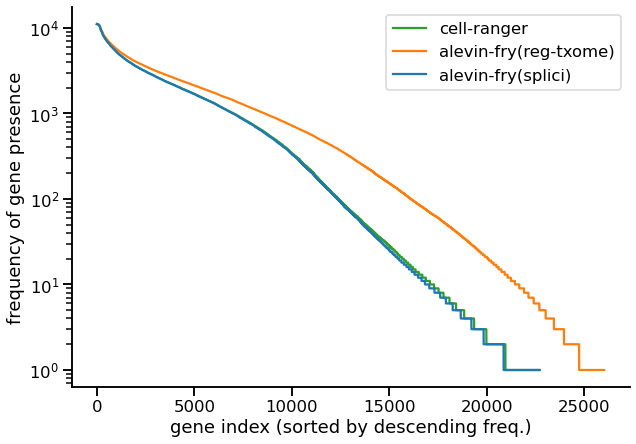
First we examine a plot that demonstrates the issue that is raised in section 2.3 of the STARsolo pre-print. Specifically, we consider plotting, for each gene g, the number of (filtered) cells e(g) in which g is expressed. The genes are placed in descending order by their frequency, and the frequency is plotted on the y-axis (log scale). Of course, it is crucial to keep in mind that since this is experimental data, we do not know the true expression profiles for each gene, and it is almost certainly true that no existing method is yet making optimal use of the data in inferring the true gene expressions. However, if pseudoalignment-to-transcriptome is inducing false positive or spurious expression, we would expect this to manifest as there being a larger number of genes that are expressed in a larger number of cells. This is what we observe in the following plot for the PBMC10k (v3) data ⁽³⁾.

Fig 1. Frequency distribution of the number of cells in which a gene is expressed.

Here, we see that Cell Ranger (the green line) produces a frequency distribution that is very closely tracked by alevin-fry using the splici transcriptome (the approach covered in this tutorial). However, if we examine the distribution for alevin-fry when using just the spliced transcriptome (orange line), then we observe that there are many more genes that are present in a higher number of cells compared to the other two approaches. Given the difference between the two alevin-fry variants, then, the most likely explanation for these added counts is that they arise from unspliced transcripts (i.e. from the intronic regions of their annotated genes). By including the intronic sequence in our index, and tracking the likely origin of each UMI, the approach using the splici transcriptome is able to report the subset of UMIs that are most likely to have arisen from mature (spliced) gene transcripts.

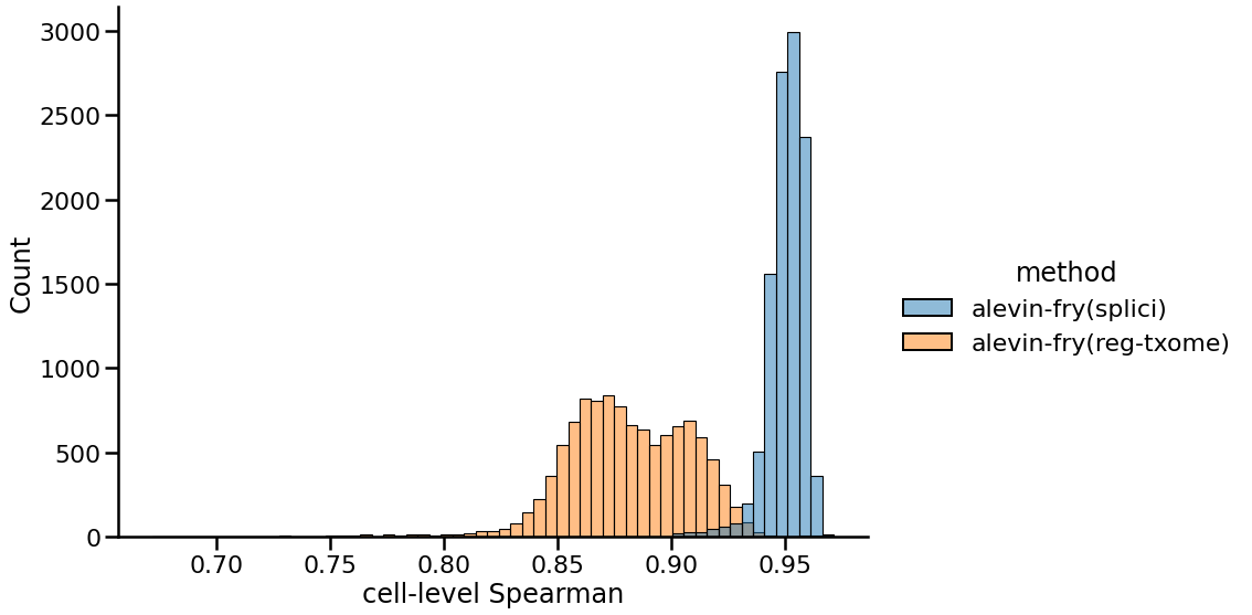
While Figure 1 illustrates the issue, it is telling us very little about the finer structure of which genes are expressed in which cells, and the effect this may have on other measures of concordance between the tools. So, next we look at the distribution of correlations between the gene expression vectors of each cell between these two processing approaches compared to the counts recorded in the pre-processed matrix provided by 10x (produced by Cell Ranger v3, in this case). Here we observe that the distribution of correlations using the splici transcriptome and USA-based quantification approach is much further to the right, concentrated around 0.95. On the other hand, the distribution of correlations when quantifying using just the spliced transcriptome is much wider, with a mean around 0.88. This suggests that the genes whose expression is truncated when using the splici transcriptome and USA-based quantification approach are quite concordant with the genes detected by the Cell Ranger pipeline for this sample. Hence, when genes are detected via UMIs associated with their spliced transcripts, these genes are still properly detected by the expanded transcriptome reference and the modified counting approach, while genes expressed primarily via intronic regions are filtered out.

Fig 2. Distribution of cell-level Spearman correlations of gene expression vectors between different approaches and Cell Ranger.

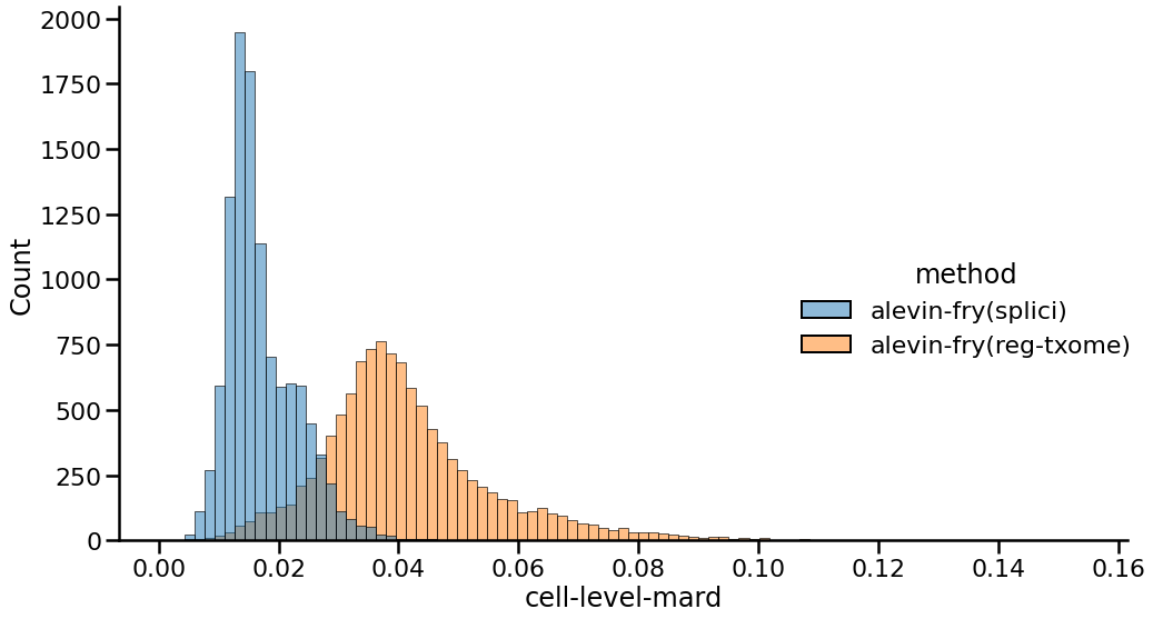
Finally, to explore the effect of this alternative quantification strategy under a different metric, we can also look at the distribution of the MARDs (Mean Absolute Relative Differences) between the gene expression vectors of each cell when comparing each method against the gene expression vectors of the Cell Ranger preprocessed matrix. Here, a lower MARD value indicates a better agreement between a pair of gene expression profiles, and so a distribution shifted further to the left indicates stronger agreement across cells. Moreover, a more peaked and less broad distribution indicates less variation in agreement.

Fig 3. Distribution of cell-level mean absolute relative differences of gene expression vectors between different approaches and Cell Ranger.

Here, the results we observe complement and concord with what we saw in Figures 1 and 2. The counts produced using the splici transcriptome and the USA-mode quantification have a mean MARD of 0.017 while those produced using the standard quantification approach against just the spliced transcriptome have a MARD of 0.041. Thus, as with the other metrics explored above, using the splici transcriptome reference and the USA-mode quantification estimates improves concordance with the Cell Ranger pipeline, which itself aligns to the genome using STAR and takes care (when performing single-cell as opposed to e.g. single-nucleus quantification) to avoid counting UMIs associated with fragments that are confidently intronic in origen in favor of the genes from which they arise.

As mentioned at the start of this tutorial, it is certainly the case that deeper investigation of these effects is warranted, both into the array of mechanisms that may cause them and into various strategies to mitigate them. It is also not yet certain if, or in what cases, an approach like that proposed here should necessarily be preferred over mapping directly to the spliced transcriptome alone. Nonetheless, there seem to be a number of benefits in the approach to the quantification of single-cell RNA-seq data described here. While we have expanded the size of our index (here, in the case of human, to ~10G) and the RAM requirements (from ~3.4G to ~12.4G), they still remain rather modest, and all of these analyses can be performed on a computer with <= 16G of RAM. Further, any reduction in speed is marginal. The entire mapping and quantification process took less than 22 minutes on this data, 16 of which was consumed by the mapping phase — which is very similar to the time taken when mapping against the standard spliced transcriptome. The peak processing memory was used during mapping, which required 12.4G of RAM; the rest of the processing steps each required <3G of RAM.

Further, this approach makes explicit certain assumptions that are implicit in a standard approach of mapping directly to the spliced transcriptome, namely the manner in which fragments arising from an unspliced transcript whose intron overlaps or shares sequence with the exon of other annotated transcripts should be accounted. It goes without saying that the genomes under study are complex, with exons of transcripts/genes falling within introns of other transcripts/genes. As seen before, preprocessing choices can greatly impact downstream inference. In this approach, as when one is following many common pipelines to perform an RNA-velocity analysis, it is made explicit which UMIs are to be associated with spliced molecules, which are to be associated with unspliced molecules, and which are ambiguous (those whose splicing status cannot be confidently determined from the information present in the experiment). The UMIs that are confidently assigned to intronic features do not go away, rather they are simply explicitly separated from the other splicing categories; hence, they can still be used in any analysis for which they may be relevant. We hope that the analysis approach presented here will help to bridge the gap between the fastest and most resource frugal preprocessing approaches and those allowing us to determine, with the greatest precision, which genes are expressing mature, spliced transcripts in single-cell RNA-seq experiments.

Notes

• While presented as a stand-alone function above, we plan to add the functionality for loading and processing quantification estimates generated in USA-mode into fishpond / tximeta in the current development cycle.

• After taking the time to read and consider the pseudoalignment-to-transcriptome issues raised in the STARsolo preprint, the work to conceptualize, develop, implement and check this approach with such quick turn-around was the effort of the whole alevin-fry team; specifically, Mohsen Zakeri, Dongze He, Avi Srivastava and Hirak Sarkar. We would also like to thank Charlotte Soneson and Mike Love for providing valuable feedback on the proposed pipeline and tutorial.

Footnotes